
If you’re anything like me, you play the Premier League’s official fantasy football game every year. And every year, by about November, you forget about it. This had me wondering – what’s the best possible team I can set on Gameweek 1 and forget about it for the rest of the season. Using data from the 2019/20 Premier League season, I set about to find the answer.
Setting Up
For this experiment, I’m using data from this github repo from user vaastav. I’ve taken the data for the 19/20 season. The analysis was carried out using the python library PuLP. PuLP is a linear programming modeller which is perfect for problems like this. We want to maximise the score of our team by choosing the variables (players) which will result in the highest score subject to certain conditions. There will be more detail below, but a great resource for understanding PuLP better can be found in this series of posts by Ben Alex Keen. I’ve carried out my analysis in a Jupyter Notebook, which you can find on my github, here.
Data Preparation
From the FPL repo above, I’ve downloaded two files – merged_gw.csv and players_raw.csv. merged_gw contains information on how each player scored in every gameweek for the season. players_raw gives information on the players, such as their position and team – stuff we’ll need later. Let’s start by tidying up merged_gw.
I’ll load the dataset in using pandas’ read_csv() function. There’s 33 columns in this dataframe, but we only need four, so I’ll make a quick subset with only the columns that contain info that we care about.
## init - load libraries
import pulp
import pandas as pd
from dfply import *

## Load in the data
gw_df = pd.read_csv("merged_gw.csv")

## Remove all unnecessary columns
gw_trim = gw_df[["name", "total_points", "GW", "value"]]
After this point, I’ll be using piping to help adjust the data into the shape we need. To enable piping, I’ve used the Dfply library, the docs of which can be found here. If you’ve used dplyr in R, this will be familiar. If not, hold tight.
Since our aim is to see what team would be the best to pick in GW1 and ignore until the end of the season, we should subset the data to only players who were avaiable to pick in GW1. We also want to know what their total score at the end of the season is. We’re being lazy, no substitutes, no changing captain, no wildcards.
## Add a column containing the final score of each player
gw_trim = (gw_trim >>
group_by(X.name) >>
mutate(finalScore = X.total_points.sum()) >>
ungroup()
)
## Only want players available to pick from the get go
## Subset to GW1 rows - this gives us initial price and only players avaiable since GW1
gw_trim = gw_trim[gw_trim["GW"] == 1]
gw_final = gw_trim.drop(["total_points", "GW"], 1)
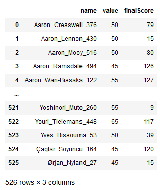
gw_final
So what is happening up there? Well, in order to get the final score of each player we are adding a column named finalScore with the mutate() function. finalScore contains the sum of the total_points column that already exists in the dataset. Above mutate in line 13 we have group_by(). We’ve grouped by player using the name column. This means when our sum function adds together the total_points values, it groups those sums by player. If we didn’t first group by player, finalScore would have identical contents in every row, just containing the full sum of all points by all players. It’s also important to ungroup() when you’re done, to prevent any accidental groupings in future analysis.
Next, the data is subset to rows that refer to GW1. This leaves only players who were available to pick at the beginning, and their price at that point. Then we drop the unnecessary columns and this is what we’re left with:
Now it’s time to add and clean the player data. Our first steps are the same – load in the data and subset to take only what we need. Here “element_type” is the name of the variable which contains a player’s position.
## Load in player data
pl_df = pd.read_csv("players_raw.csv")
pl_trim = pl_df[["first_name",  "second_name", "element_type",  "id",  "team"]]
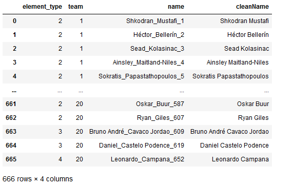
In the player’s dataset, we have a first_name column, a second_name column, and an id column. As you can see in the screenshot of our gw_final dataframe above, all three of those datapoints are contained in one column titled name. In order to make it possible to join our datasets, we need a column in the same format. I’m also adding a column cleanName which is exactly what it sounds like.
In order to concatenate the id variable onto the end of the players’ names, it needs to be changed from an integer to a string. This is where I wish I did the cleaning in R. I’ve used seven different methods to convert the column type to string, all of which produced a warning that no amount of reading docs/asking for help on reddit could solve. If you can explain why this is giving me a SettingWithCopyWarning, please reach out. I’ve only included one below, but all seven attempts I made are in the notebook on my github, if you’re curious.
## Convert ID to string to allow concatenation
pl_trim["id"] = pl_trim.loc[:,"id"].astype(str)

## Add name columns
pl_trim = (pl_trim >>
           mutate(name = X.first_name + "_" + X.second_name + "_" + X.id) >>
           mutate(cleanName = X.first_name + " " + X.second_name) >>
           drop(X.first_name, X.second_name, X.id)
          )
Now, our data looks like this:
So we’re ready to combine these into one.
combined_df = (gw_final >> left_join(pl_trim, by = "name"))
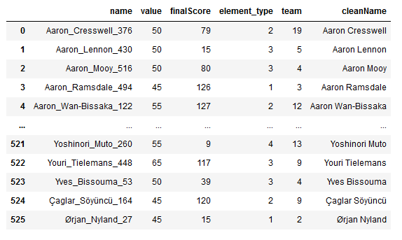
I’ve used a left join here as gw_final is the “A” dataset, and this is the one that is limited to players we can actually choose in GW1. We’ve joined by name as it is the closest thing we have to a primary key here. The combined dataset looks likes this:
Time for PuLP
The first thing we want to do is figure out what our variables are. As we’re picking a team, it’s clear that the players are our variables. We want to create a dictionary that contains all of our players and a value of 0 if they are not selected in the team, and a value of 1 if they are selected. We do this using the pulp.LpVariable.dict() function.
## Set variables
x = pulp.LpVariable.dict("player", range(0, len(combined_df)),
                        0,1, cat=pulp.LpInteger)
Now, we need to determine our objective function. This is the function we either want to minimise or maximise. Well, we want the highest score we can get. So it makes sense that we want to maximise by summing the finalScore of each player. We can do this by initialising the problem with pulp.LpProblem(), and then adding our function.
prob = pulp.LpProblem("FantasyFootball", pulp.LpMaximize)
prob += pulp.lpSum(combined_df["finalScore"][i] * x[i] for i in range(0, len(combined_df)))
Finally, we need to figure out our constraints. There aren’t too many to worry about here.
- We need exactly 11 players
- We need exactly 1 goalkeeper
- We need 3-5 defenders
- We need 3-5 midfielders
- We need 1-3 forwards
- Our budget is 100m (for now)
Let’s add these constraints to our problem one at a time.
## Max 11 players
prob += sum(x[i] for i in range(0, len(combined_df))) ==  11
As mentioned above, each of our variables is stored in a dictionary, where 0 represents a player who is not chosen, and 1 represents a player who has been chosen. In the above line of code we are saying that when the value of all of the 1s or 0s are summed together, it must equal exactly 11. This ensures that we have exactly 11 players in our team. Let’s do the same for limiting our number of goalkeepers to 1.
## One goalkeeper
prob  += sum(x[i] for i in range(0, len(combined_df)) if combined_df["element_type"][i] == 1) == 1
Here, we are stating that the sum of 1s and 0s for all players who appear in our combined_df as a goalkeeper (element type 1) must equal exactly 1. We’re checking our variables index i versus our combined_df index i to checkthe players’ position. Let’s do it again for the other positions.
## Three to Five Defenders
prob  += sum(x[i] for i in range(0, len(combined_df)) if combined_df["element_type"][i] == 2) >= 3
prob  += sum(x[i] for i in range(0, len(combined_df)) if combined_df["element_type"][i] == 2) <= 5

## Three to Five Midfielders
prob  += sum(x[i] for i in range(0, len(combined_df)) if combined_df["element_type"][i] == 3) >= 3
prob  += sum(x[i] for i in range(0, len(combined_df)) if combined_df["element_type"][i] == 3) <= 5

## One to Three Attackers
prob  += sum(x[i] for i in range(0, len(combined_df)) if combined_df["element_type"][i] == 4) >= 1
prob  += sum(x[i] for i in range(0, len(combined_df)) if combined_df["element_type"][i] == 4) <= 3
Finally, our budget constraint. We said above our budget is 100 million (for now). The reason this is for now is that we do also need to buy some subs. But don’t worry, as we’re lazy and never use any of our subs, it does not matter who we pick. So, let’s just pick the cheapest player in each position. That’s a 4m GK, a 4m defender, a 5m midfielder, and a 4.5m forward – a total of 17.5m. To save ourself the trouble of trying to encode “Pick the 11 best players and then four cheap ones”, let’s just reduce our budget by 17.5m and only care about the starting 11.
# 100MM budget (100mil in dataset is 1000)
# This does not account for subs however
# Decrease budget by the price of the cheapest player in each pos
# 4 for GK, 4 for DEF, 5 for MID, 4.5 for FW - 17.5 total
prob += sum(x[i] * combined_df["value"][i] for i in range(0, len(combined_df))) <= 825  # total cost
Okay, let’s see if we have a team!
print(prob.solve()) # Outputs 1 if successful
print(pulp.LpStatus[prob.status]) # Outputs "Optimal" if... well, optimal
print(pulp.value(prob.objective)) # Shows us our points total

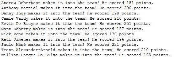
We have a team! A good team! A team that scored 2170 points (and we haven’t even chosen our captain yet). Let’s see who made the cut.
for i in range(0, len(combined_df)):
    if pulp.value(x[i]) == 1:
        print("{player} makes it into the team! He scored {points} points.".format(player = combined_df["cleanName"][i], points = combined_df["finalScore"][i]))
When PuLP solved the problem, it changed the values in our dictionary to show our starting 11 encoded as 1s. The above loop looks at each entry to our dictionary and prints out those who made the cut.
Since these are printing in alphabetical order, it’s a bit hard to see the structure of our team. I’ll make a pandas dataframe to store our final team, which I’ll sort by position to easier see our formation. I can also double our best scoring player’s points and put a (C) beside his name to note him as captain. My method here isn’t the prettiest, and also gives a SettingWithCopyWarning, so please leave a comment if you can help me tidy this up.
squad = pd.DataFrame()
for i in range(0, len(combined_df)):
    if pulp.value(x[i]) != 0:
        squad = squad.append(combined_df[i:i+1], ignore_index = True)
squad = squad.sort_values(by = ["element_type"])

## Double the best player's score (captain)
squad["finalScore"][squad["finalScore"] == max(squad["finalScore"])] = 2 * max(squad["finalScore"])
squad["cleanName"][squad["finalScore"] == max(squad["finalScore"])] = squad["cleanName"][squad["finalScore"] == max(squad["finalScore"])] + "(C)"
Let’s take a look at our squad.

I’ve also written a function to print our squad a little more nicely. I won’t include it here, as there is a lot you would need to change should you play around with this using different constraints. It is still in the notebook on github however.
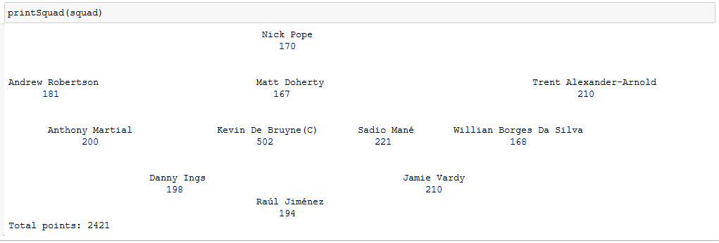
So there we are. The best lazy FPL team of last season would have netted you 2,421 points. A seriously impressive total, considering the winner of FPL 2019/20 had 2,557 points. That’s only 3.5 points per week better!
Next, I just need to find a way to make a football pun/team name generator. Until then, maybe learn how to simulate football games in R using xG values.
